Download this notebook from github.

Advanced explanation for RadarSat2

Contrary to Sentinel-1, RadarSat-2 doesn’t have the notion of multi dataset

[1]:

import xsar
import geoviews as gv
import holoviews as hv
import geoviews.feature as gf
hv.extension('bokeh')
path = xsar.get_test_file('RS2_OK135107_PK1187782_DK1151894_SCWA_20220407_182127_VV_VH_SGF')

Open a dataset

[6]:

# Define the resolution to load the dataset at a lower resolution (if not specified or None, the dataset is loaded at high resolution)
resolution = '1000m'

# Instanciate a RadarSatDataset object
rs2ds = xsar.RadarSat2Dataset(dataset_id=path, resolution=resolution)

Get the Dataset object

[7]:

rs2ds

[7]:

<RadarSat2Dataset full coverage object>

Access the metadata object from the Dataset object

[8]:

rs2ds.sar_meta

[8]:

<BlockingActorProxy: RadarSat2Meta>

Access the dataset

In this dataset, we can find variables like latitude, longitude, look up tables (before and after denoising), incidence…

[9]:

rs2ds.dataset

[9]:

<xarray.Dataset>
Dimensions:          (pol: 2, line: 513, sample: 530)
Coordinates:
  * pol              (pol) <U2 'VV' 'VH'
  * line             (line) float64 9.5 29.5 49.5 ... 1.023e+04 1.025e+04
  * sample           (sample) float64 9.5 29.5 49.5 ... 1.057e+04 1.059e+04
Data variables: (12/23)
    digital_number   (pol, line, sample) uint16 dask.array<chunksize=(1, 513, 530), meta=np.ndarray>
    lines_flipped    bool False
    samples_flipped  bool True
    sampleSpacing    float64 1e+03
    lineSpacing      float64 1e+03
    sigma0_raw       (pol, line, sample) float64 dask.array<chunksize=(1, 513, 530), meta=np.ndarray>
    ...               ...
    time             (line) datetime64[ns] dask.array<chunksize=(513,), meta=np.ndarray>
    latitude         (line, sample) float64 dask.array<chunksize=(513, 530), meta=np.ndarray>
    longitude        (line, sample) float64 dask.array<chunksize=(513, 530), meta=np.ndarray>
    altitude         (line, sample) float64 dask.array<chunksize=(513, 530), meta=np.ndarray>
    incidence        (line, sample) float64 dask.array<chunksize=(513, 530), meta=np.ndarray>
    elevation        (line, sample) float64 dask.array<chunksize=(513, 530), meta=np.ndarray>
Attributes: (12/18)
    product_path:           /tmp/RS2_OK135107_PK1187782_DK1151894_SCWA_202204...
    satellite:              RADARSAT-2
    inputDatasetId:         /Fred/RSAT-2/610044P
    rawDataStartTime:       2022-04-07T18:21:27.688416000
    satelliteHeight_units:  m
    satelliteHeight:        800612.0083192665
    ...                     ...
    stop_date:              2022-04-07 18:22:44.030964
    footprint:              POLYGON ((168.8147284622835 -19.82390747944243, 1...
    coverage:               515km * 530km (line * sample )
    pixel_line_m:           50.0
    pixel_sample_m:         50.0
    approx_transform:       |-0.00,-0.00, 168.85|\n|-0.00, 0.00,-19.85|\n| 0....

Variables lines_flippedand samples_flipped are added to the dataset to know if these have been flipped (in order to follow xsar convention)

Alternatives solutions to open dataset and datatree

[10]:

# Open dataset
xsar.open_dataset(path, resolution=resolution)

[10]:

<xarray.Dataset>
Dimensions:          (pol: 2, line: 513, sample: 530)
Coordinates:
  * pol              (pol) <U2 'VV' 'VH'
  * line             (line) float64 9.5 29.5 49.5 ... 1.023e+04 1.025e+04
  * sample           (sample) float64 9.5 29.5 49.5 ... 1.057e+04 1.059e+04
Data variables: (12/23)
    digital_number   (pol, line, sample) uint16 dask.array<chunksize=(1, 513, 530), meta=np.ndarray>
    lines_flipped    bool False
    samples_flipped  bool True
    sampleSpacing    float64 1e+03
    lineSpacing      float64 1e+03
    sigma0_raw       (pol, line, sample) float64 dask.array<chunksize=(1, 513, 530), meta=np.ndarray>
    ...               ...
    time             (line) datetime64[ns] dask.array<chunksize=(513,), meta=np.ndarray>
    latitude         (line, sample) float64 dask.array<chunksize=(513, 530), meta=np.ndarray>
    longitude        (line, sample) float64 dask.array<chunksize=(513, 530), meta=np.ndarray>
    altitude         (line, sample) float64 dask.array<chunksize=(513, 530), meta=np.ndarray>
    incidence        (line, sample) float64 dask.array<chunksize=(513, 530), meta=np.ndarray>
    elevation        (line, sample) float64 dask.array<chunksize=(513, 530), meta=np.ndarray>
Attributes: (12/18)
    product_path:           /tmp/RS2_OK135107_PK1187782_DK1151894_SCWA_202204...
    satellite:              RADARSAT-2
    inputDatasetId:         /Fred/RSAT-2/610044P
    rawDataStartTime:       2022-04-07T18:21:27.688416000
    satelliteHeight_units:  m
    satelliteHeight:        800612.0083192665
    ...                     ...
    stop_date:              2022-04-07 18:22:44.030964
    footprint:              POLYGON ((168.8147284622835 -19.82390747944243, 1...
    coverage:               515km * 530km (line * sample )
    pixel_line_m:           50.0
    pixel_sample_m:         50.0
    approx_transform:       |-0.00,-0.00, 168.85|\n|-0.00, 0.00,-19.85|\n| 0....

[11]:

# Open datatree
xsar.open_datatree(path, resolution=resolution)

[11]:

<xarray.DatasetView>
Dimensions:  ()
Data variables:
    *empty*
Attributes: (12/18)
    product_path:           /tmp/RS2_OK135107_PK1187782_DK1151894_SCWA_202204...
    satellite:              RADARSAT-2
    inputDatasetId:         /Fred/RSAT-2/610044P
    rawDataStartTime:       2022-04-07T18:21:27.688416000
    satelliteHeight_units:  m
    satelliteHeight:        800612.0083192665
    ...                     ...
    stop_date:              2022-04-07 18:22:44.030964
    footprint:              POLYGON ((168.8147284622835 -19.82390747944243, 1...
    coverage:               515km * 530km (line * sample )
    pixel_line_m:           50.0
    pixel_sample_m:         50.0
    approx_transform:       |-0.00,-0.00, 168.85|\n|-0.00, 0.00,-19.85|\n| 0....

How to apply calibration?

All the operation below are already performed by default for GRD products. So, what is following is a simple explanation about how is made calibration.

Load digital numbers

load_digital_number is a function that allows to load digital numbers from tiff files at chosen resolution and return it as a DataArray. Resampling is made thanks to rasterio.open(tiff_file).read. For dual pol products, there is a tiff file for each pol. So that digital numbers are computed for both pol. Posting of lines and samples is computed thanks to Affine.translation and Affine.scale.

[12]:

from xradarsat2 import load_digital_number
import rasterio

#Define resampling method (here it is the root mean square from rasterio)
resampling = rasterio.enums.Resampling.rms

#Define the chunks size for line and samples
chunks = {'line': 5000, 'sample': 5000}

[13]:

dn_low_res = load_digital_number(rs2ds.sar_meta.dt, resolution=resolution, resampling=resampling, chunks=chunks)['digital_numbers'].ds
dn_low_res

[13]:

<xarray.DatasetView>
Dimensions:         (pol: 2, line: 513, sample: 530)
Coordinates:
  * pol             (pol) <U2 'VV' 'VH'
  * line            (line) float64 9.5 29.5 49.5 ... 1.023e+04 1.025e+04
  * sample          (sample) float64 9.5 29.5 49.5 ... 1.057e+04 1.059e+04
Data variables:
    digital_number  (pol, line, sample) uint16 dask.array<chunksize=(1, 513, 530), meta=np.ndarray>

Get the raw normalized radar cross section

_apply_calibration_lut is a method that applies a calibration look up table to digital numbers to compute gamma0, beta0 and sigma0 (depending on the variable name passed in argument) and return the result as a DataArray. It first get the high resolution calibration look up table. But it isn’t at the good resolution (already high resolution). So, this functions uses another one named _resample_lut_values. Once the calibration look up table is at the good resolution, we can apply the following formula :

\[\frac{(digitalNumbers^2)+offset}{Gain}\]

Reference : Radarsat2 Product Format Definition (7.2) : https://earth.esa.int/eogateway/documents/20142/0/Radarsat-2-Product-Format-Definition.pdf/1ca0cf1e-5a15-a29b-6187-9e5cb1650048#page=77

_resample_lut_values uses RectBivariateSplinefor the interpolation, but it is necessary that data is expressed as a 2D vector. Here, calibration look up tables are expressed as 1D vector (range sample). Consequently, we need to convert these in 2D (adding an azimuth dimension dependency) before applying the interpolation. Conversion is made thanks to numpy.tile, using the low resolution lines expressed in the geolocation grid part of the reader; reducing the calculation. A template of a DataArray that uses the posting of digital numbers (with applied resolution) is given on this interpolation function so the result is now at the right resolution.

Different resampling method were tried such as scipy.ndimage.gaussian_filter1d that had the convenience to accept 1d vectors. Data was computed with this function and the chosen posting was this of digital numbers. But in order to be homogenous with other operations made in xsar, we chose to keep the solution with RectBivariateSpline.

[14]:

sigma0_raw = rs2ds._apply_calibration_lut('sigma0').sigma0_raw
sigma0_raw

[14]:

<xarray.DataArray 'sigma0_raw' (pol: 2, line: 513, sample: 530)>
dask.array<where, shape=(2, 513, 530), dtype=float64, chunksize=(1, 513, 530), chunktype=numpy.ndarray>
Coordinates:
  * line     (line) float64 9.5 29.5 49.5 69.5 ... 1.021e+04 1.023e+04 1.025e+04
  * sample   (sample) float64 9.5 29.5 49.5 ... 1.055e+04 1.057e+04 1.059e+04
  * pol      (pol) <U2 'VV' 'VH'

[15]:

import matplotlib.pyplot as plt

[16]:

plt.figure(figsize=(13, 6))

plt.subplot(1, 2, 1)
sigma0_raw_cross = sigma0_raw.sel(pol='VH')
plt.pcolor(sigma0_raw_cross, vmax=0.02, cmap='Greys_r')
plt.title('sigma0_raw VH')
plt.xlabel('samples')
plt.ylabel('lines')
plt.colorbar()

plt.subplot(1, 2, 2)
sigma0_raw_co = sigma0_raw.sel(pol='VV')
plt.pcolor(sigma0_raw_co, vmax=0.7, cmap='Greys_r')
plt.title('sigma0_raw VV')
plt.xlabel('samples')
plt.ylabel('lines')
plt.colorbar()

[16]:

<matplotlib.colorbar.Colorbar at 0x7fb2deb433a0>

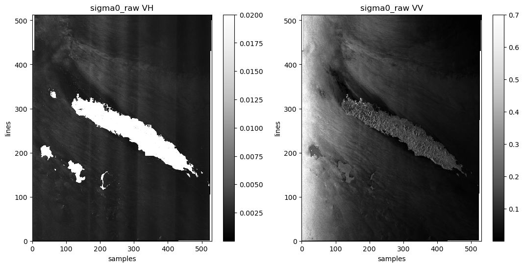
How to apply denoising ?

All the operation below are already performed by default for GRD products. So, what is following is a simple explanation about how is made denoising.

How to get the Noise Equivalent Sigma Zero ?

NoiseLevelValues at low resolution are extracted from product.xml and then located in the datatree of the metadata (dt['radarParameters']). They are already calibrated so we don’t have to apply a calibration on theseThey are expressed in dB, and are given with a pixelFirstNoiseValue and a stepSize. With these information we have now to build the noise_lut. The first thing to do is to convert the NoiseLevelValues in linear :

\[NoiseLevelValues_{linear} = 10^\frac{NoiseLevelValues_{dB}}{10}\]

Right now we compute the nesz thanks to the following documentation : https://earth.esa.int/eogateway/documents/20142/0/Radarsat-2-Product-Format-Definition.pdf/1ca0cf1e-5a15-a29b-6187-9e5cb1650048#page=70

[17]:

nesz_low_res = rs2ds._interpolate_for_noise_lut('sigma0')
nesz_low_res

[17]:

<xarray.DataArray "Delayed('RectBivariateSpline-ac6cfb5b-3413-4e78-83-971e03872ee53eeba910249e53cf7a69" (
                                                                                                         line: 513,
                                                                                                         sample: 530)>
dask.array<Delayed('RectBivariateSpline-ac6cfb5b-3413-4e78-83, shape=(513, 530), dtype=float32, chunksize=(513, 530), chunktype=numpy.ndarray>
Coordinates:
  * line     (line) float64 9.5 29.5 49.5 69.5 ... 1.021e+04 1.023e+04 1.025e+04
  * sample   (sample) float64 9.5 29.5 49.5 ... 1.055e+04 1.057e+04 1.059e+04

[18]:

plt.pcolor(nesz_low_res, vmax=0.005, cmap='Greys_r')
plt.title('nesz')
plt.xlabel('samples')
plt.ylabel('lines')
plt.colorbar()

[18]:

<matplotlib.colorbar.Colorbar at 0x7fb2ce766bc0>

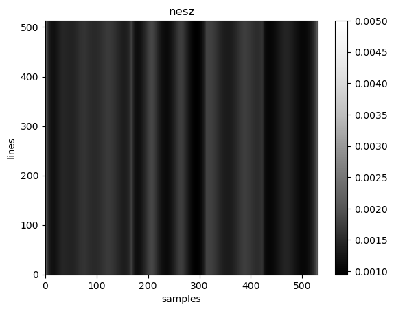
How to get the noise substracted Sigma0

Right now we only have to substract the noise_lut to the raw normalized radar cross section. It is made with the function _add_denoised, that add the variables to the RadarSat2Dataset.dataset

[19]:

sigma0 = sigma0_raw - nesz_low_res
sigma0

[19]:

<xarray.DataArray (pol: 2, line: 513, sample: 530)>
dask.array<sub, shape=(2, 513, 530), dtype=float64, chunksize=(1, 513, 530), chunktype=numpy.ndarray>
Coordinates:
  * line     (line) float64 9.5 29.5 49.5 69.5 ... 1.021e+04 1.023e+04 1.025e+04
  * sample   (sample) float64 9.5 29.5 49.5 ... 1.055e+04 1.057e+04 1.059e+04
  * pol      (pol) <U2 'VV' 'VH'

Comparison between noised sigma0 and noised substracted sigma0

[20]:

plt.figure(figsize=(26, 12))

sigma0_cross = sigma0.sel(pol='VH')
sigma0_co = sigma0.sel(pol='VV')

plt.subplot(2,2,1)
plt.pcolor(sigma0_raw_cross, vmax=0.02, cmap='Greys_r')
plt.title('Sigma0 VH with noise')
plt.xlabel('samples')
plt.ylabel('lines')
plt.colorbar()

plt.subplot(2,2,3)
plt.pcolor(sigma0_cross, vmax=0.02, cmap='Greys_r')
plt.title('Sigma0 VH without noise')
plt.xlabel('samples')
plt.ylabel('lines')
plt.colorbar()

plt.subplot(2,2,2)
plt.pcolor(sigma0_raw_co, vmax=0.7, cmap='Greys_r')
plt.title('Sigma0 VV with noise')
plt.xlabel('samples')
plt.ylabel('lines')
plt.colorbar()

plt.subplot(2,2,4)
plt.pcolor(sigma0_co, vmax=0.7, cmap='Greys_r')
plt.title('Sigma0 VV without noise')
plt.xlabel('samples')
plt.ylabel('lines')
plt.colorbar()

[20]:

<matplotlib.colorbar.Colorbar at 0x7fb2a563ecb0>

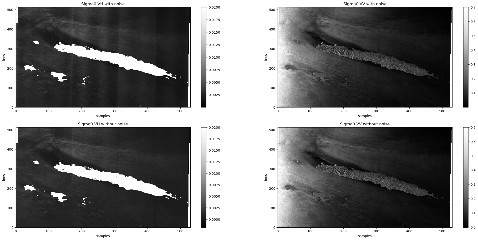
How to get the incidence ?

Radarsat2 product format definition (7.2) provides a formula of look up tables, depending on the incidence. We already have information about look up tables, so we determine incidence with these look up tables:

\[Incidence = \arctan{\frac{\gamma}{\beta}}\]

reference link : https://earth.esa.int/eogateway/documents/20142/0/Radarsat-2-Product-Format-Definition.pdf/1ca0cf1e-5a15-a29b-6187-9e5cb1650048#page=78

We have the choice between 2 types of look up tables: denoised and not denoised. We have chosen to determine incidence with not denoised look up tables. This computation is made by the function _load_incidence_from_lut that returns a DatArray

[21]:

incidence = rs2ds._load_incidence_from_lut()
incidence

[21]:

<xarray.DataArray (line: 513, sample: 530)>
dask.array<degrees, shape=(513, 530), dtype=float64, chunksize=(513, 530), chunktype=numpy.ndarray>
Coordinates:
  * line     (line) float64 9.5 29.5 49.5 69.5 ... 1.021e+04 1.023e+04 1.025e+04
  * sample   (sample) float64 9.5 29.5 49.5 ... 1.055e+04 1.057e+04 1.059e+04

How to get the elevation ?

To get the incidence, we apply a formula :

\[\theta = \arcsin{[\sin{(Incidence)} . \frac{r}{r + h}]}\]

\[( r \text{ is the earth radius} , h \text{ is the orbit altitude} )\]

Reference : Data Products Specifications (https://asf.alaska.edu/wp-content/uploads/2019/03/r1_prod_spec.pdf#page=47)

2 variables give orbit altitude so we considered theSatelliteHeight (and not thealtitude). RadarSat2Dataset._load_elevation_from_lut permit to calculate the elevation (in degrees).

[22]:

elevation = rs2ds._load_elevation_from_lut()
elevation

[22]:

<xarray.DataArray (line: 513, sample: 530)>
dask.array<degrees, shape=(513, 530), dtype=float64, chunksize=(513, 530), chunktype=numpy.ndarray>
Coordinates:
  * line     (line) float64 9.5 29.5 49.5 69.5 ... 1.021e+04 1.023e+04 1.025e+04
  * sample   (sample) float64 9.5 29.5 49.5 ... 1.055e+04 1.057e+04 1.059e+04